GrainGrowth 2D
ENAR

Two-Dimensional Grain Growth Simulation

Developing MATLAB code to simulate 2D grain growth

Simulated grain map at the selected step
Step
0 MCS
Grain count
0
Mean diameter
0 cells

Grain count vs. Monte Carlo steps (MCS)

Mean equivalent diameter (cells) vs. MCS

Fewer than six Six More than six

Figure 1. Grain maps exported by the GrainGrowth2D application from MATLAB in micrograph style, from a saved run: a 256 × 256 lattice starting from 1,024 nuclei, with the kernel defaults (eight neighbours, kT = 0.5). Drag the slider or click either curve to jump to any step.

Abstract

This project develops a MATLAB application that simulates grain growth in a two-dimensional section of a polycrystalline metal using the Potts model and the Monte Carlo method. The user selects the alloy and processing conditions; the application tracks boundary migration, measures grain count, grain diameter and the ASTM grain size number, and estimates strength through the Hall–Petch relation. In version 1.7.0 the simulation kernel was tested against three established laws: shrinkage of a circular grain at a constant rate, the von Neumann–Mullins law, and the f−1/2 scaling of the limiting grain size under two-dimensional particle pinning.

1Why do grains grow?

After solidification or recrystallisation, a metal consists of grains separated by boundaries that carry excess energy. On heating, the total boundary energy decreases as boundaries shorten, so boundaries migrate towards their centres of curvature: small grains shrink and disappear, and the mean grain size increases with time.

This is visible directly in Figure 1: the grain count falls from 1043 to 476 over 500 steps, and the mean equivalent diameter rises from 8.6 to 12.3 cells.

Switch on colouring by number of sides in the same figure. Grains with fewer than six sides are mostly small and shrinking, while grains with more than six sides grow at their expense. This rule was formulated by von Neumann and Mullins, and we test it quantitatively in Section 4.

2One Monte Carlo step

The sample is divided into a square lattice, and each cell carries a number identifying the grain it belongs to. The energy of a cell is the number of its eight neighbours that belong to a different grain. In each attempt a cell is chosen, the state of one of its neighbours is proposed for it, and the change is accepted according to the Metropolis rule. One attempt per lattice cell makes one Monte Carlo step, abbreviated MCS.

Proposed state
B
Unlike neighbours before
5
Unlike neighbours after
4
Energy change ΔE
−1

Acceptance probability P = min(1, e−ΔE/kT) = 1

Figure 2. A single attempt. The central cell, outlined with a dashed line, belongs to grain A. Click a neighbour to propose its state, and change kT to see how the simulation temperature affects the acceptance probability. Fuller explanation of the model

3Effect of cementite particles

In low-carbon steel, small cementite particles are distributed within the ferrite. The application represents them as fixed cells that never change. When a boundary reaches a particle it becomes attached and needs a larger driving force to break away, so growth slows and then stops at a limiting size. This is known as Zener pinning.
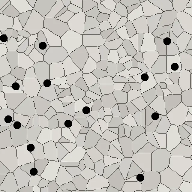
Magnified field showing cementite particles in black on grain boundaries
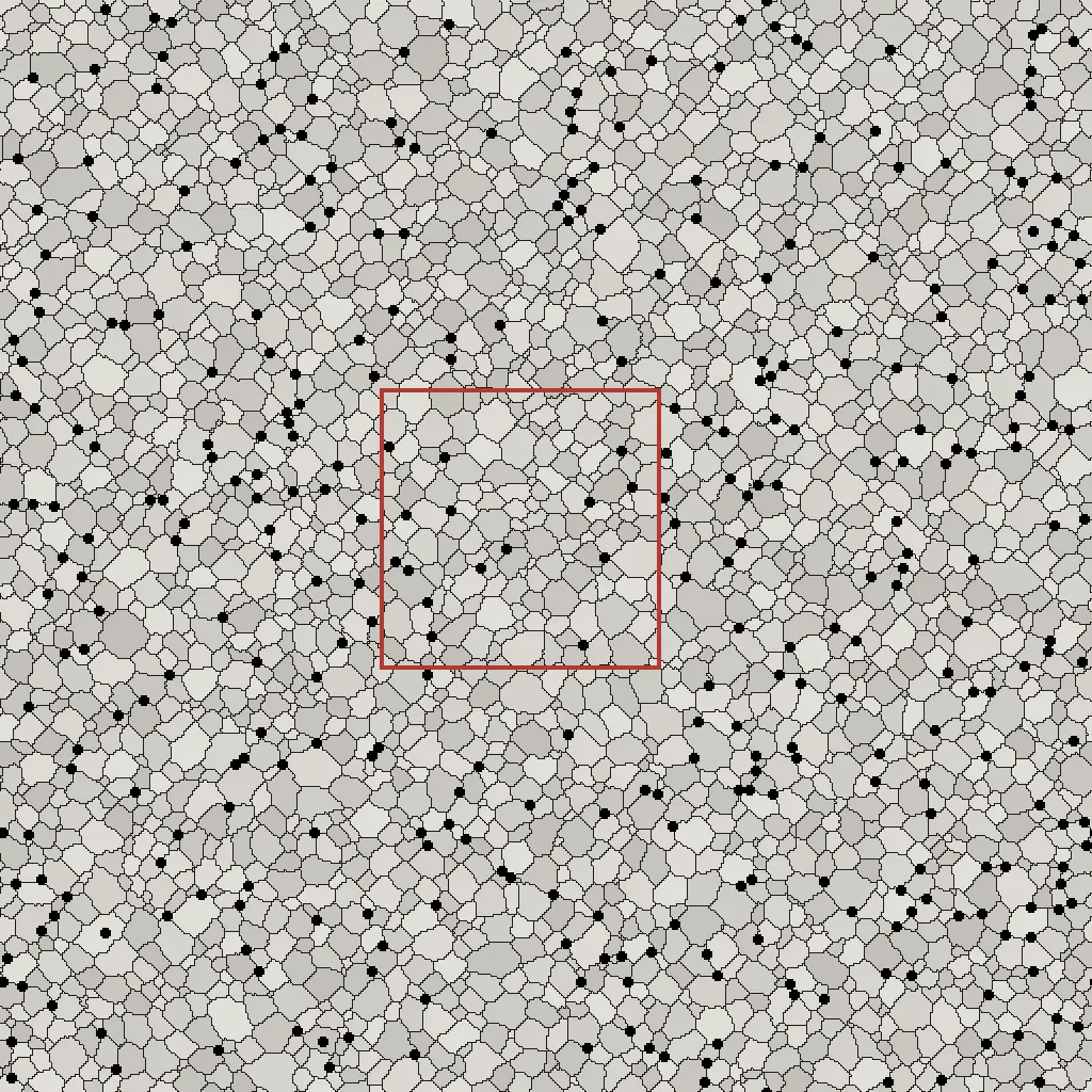
The full 512 × 512-cell field, with the magnified region outlined in red
Step
0 MCS
Grain count in the full field
0
Particles touching a boundary
0
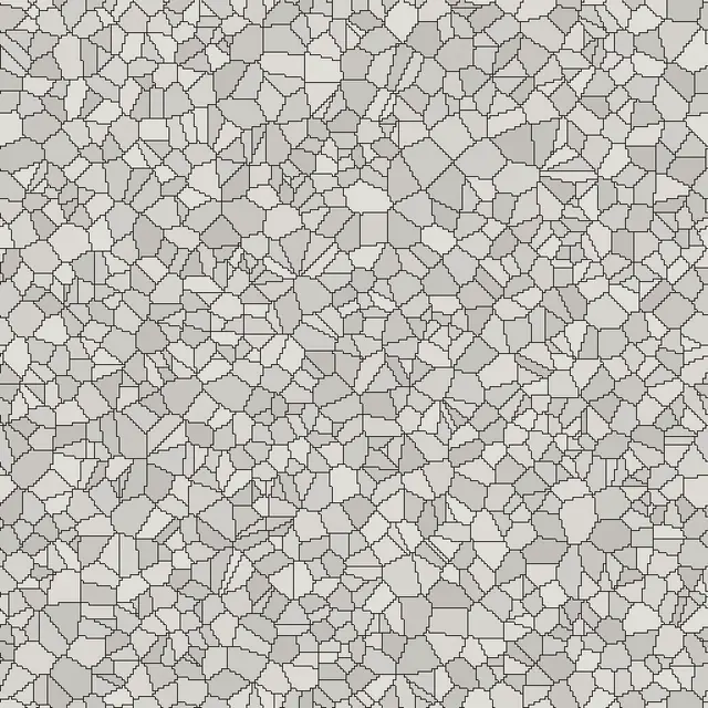
Figure 3. A saved run of an Fe–C alloy with 0.2 wt.% carbon at 923 K, on a 512 × 512 lattice in which particles occupy 2.9% of the area. The large image is a 128 × 128-cell magnified field in the application's zoomed view; its position is outlined in red on the full field. All images were exported from MATLAB.

In Figure 3 the boundaries tend to settle at the particles. After 300 steps, 99% of the particles touch a boundary between two or more grains, compared with 93% at the start, and the grain count has fallen from 4335 to 2554.

4Model versus theory

Before any applied result can be trusted, the kernel must show that it reproduces established laws of two-dimensional grain growth. Three tests were run with the same kernel, without any modification.

01000200030000100020003000MCSArea (sites)

aShrinkage of a circular grain

A grain of radius 30 cells inside one large grain. Its area decreases linearly at 0.923 cells per MCS with a coefficient of determination R² = 0.9985; it vanishes at 3030 MCS and stays round, with a maximum-to-minimum radius ratio of 1.07.

345678910−0.400.40.8Number of sides ndA/dt (sites/MCS)n0 = 5.86

bThe von Neumann–Mullins law

Mean rate of area change for each number of sides, in the colours of Figure 1. The line crosses the axis at n0 = 5.86 against the theoretical value of 6, from 261,338 observations on a 384 × 384 lattice.

0.020.040.080.1661016Particle fraction f (log)D_lim (cells, log)slope −0.518−0.5 reference

cZener pinning in two dimensions

The larger the particle fraction f, the smaller the size at which growth stops. The slope is −0.518 against the expected two-dimensional value of −0.5, from three points that reached stagnation. The open point (f = 0.02) had not stagnated by 3000 MCS and was excluded from the fit.

Figure 4. Kernel tests in version 1.7.0. Simulation result Fit Theoretical value

5The application

The application runs on MATLAB R2024b with lattices up to 512 × 512 cells. It includes five binary alloys (Fe–C, Al–Cu, Mg–Al, Ni–Al and Cu–Zn) and four studies of multicomponent alloys (CrFeNi, CoNiCr, CoNiMn and FeCoNiCrMn). Every version passes a release test of 52 suites and 512 check groups.

  1. Choose the alloy and enter the composition, temperature and duration.
  2. Set the lattice and random seed, then run the simulation.
  3. Explore the result at any step: the map, grain count and diameter, ASTM number, and the Hall–Petch estimate.
  4. Export microstructure images at 600 dpi, data tables and the settings log.
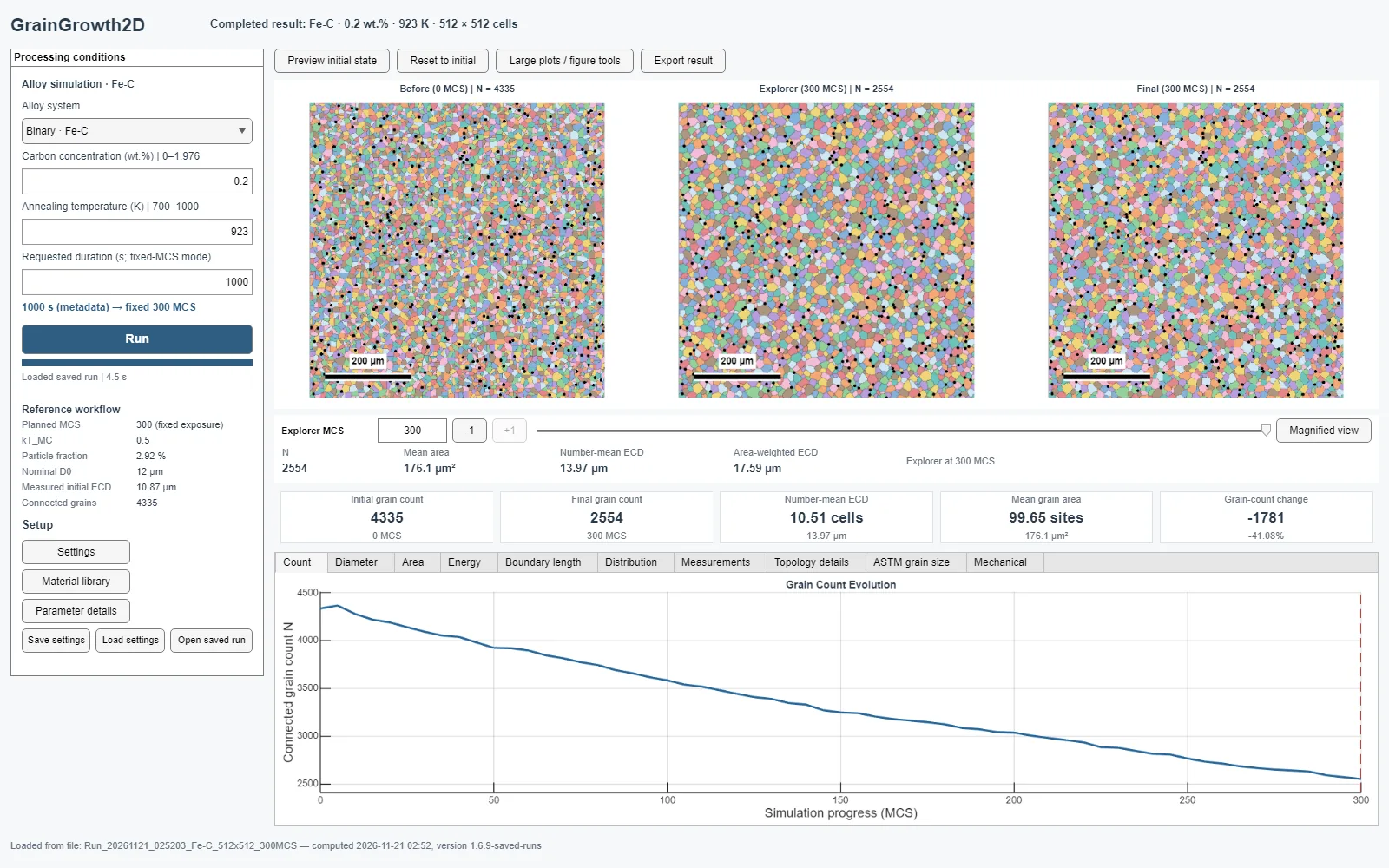
The GrainGrowth2D interface after opening the saved Fe–C run at 300 MCS
Figure 5. The application interface after opening the saved Fe–C run of Figure 3, at 300 MCS: before, intermediate and final maps, the measurements, and the grain-count curve.

6References

  1. Huang, Y.-C.; Su, C.-H.; Wu, S.-K.; Lin, C. A Study on the Hall–Petch Relationship and Grain Growth Kinetics in FCC-Structured High/Medium Entropy Alloys. Entropy 2019, 21(3), 297. doi:10.3390/e21030297
  2. Schneider, M.; Laplanche, G. Data in Brief 34 (2021) 106712, Table 1. doi:10.1016/j.dib.2020.106712
  3. Korbuly, B. et al. Grain coarsening in two-dimensional phase-field models with an orientation field. arXiv:1704.04059
  4. Martine La Boissonière, J.; Choksi, R.; Barmak, K.; Esedoğlu, S. Statistics of grain growth: experiment versus the Phase-Field-Crystal and Mullins models. arXiv:1811.11900
  5. Beenakker, C. W. J. Numerical simulation of a coarsening two-dimensional network. Phys. Rev. A 37 (1988) 1697.

Full list of references and sources of alloy values